$k$ 近邻

$k$ 近邻是一种简单的分类方法，它的基本思想是：如果一个样本在特征空间中的$k$个最相似（即特征空间中最邻近）的样本中的大多数属于某一个类别，则该样本也属于这个类别。

$k$ 近邻分类器

该算法的主要流程如下：

• 计算测试样本 $\overline{x}$ 与训练集中每个样本 $x_i$ 的距离 $d(\overline{x},x_i)$，这里的距离计算函数 $d(x,y)$ 是距离度量函数的一种，可以参考此篇文章。
• 对于所有距离值进行排序，找到距离最近的 $k$ 个样本。
• 统计这 $k$ 个样本中每个类别的个数，选择个数最多的类别分配给 $\overline{x}$。

在这一算法中，我们一般将 $k$ 取奇数，防止平局。当 $k$ 较小时，对噪声敏感，整体模型变得复杂，容易过拟合；当 $k$ 较大时，对噪声不敏感，模型变得简单，容易欠拟合。

特别地，当 $k=1$ 时，该算法称为最近邻算法。

$k$ 近邻分类器的错误率

对于最近邻分类器，如果测试样本为 $\mathbf{x}$，其最近邻样本为 $\mathbf{z}$，则有：

$$P(err)=1-{\mathrm{\Sigma }}_{c\in \mathcal{Y}}P(c|\mathbf{x})P(c\mid \mathbf{z})$$

此外，虽然看起来简单，但是如果假设样本独立同分布，那么最近邻分类器的泛化错误率居然不超过贝叶斯最优分类器的错误率的两倍！

$k$ 近邻回归

除了分类问题，$k$ 近邻还可以用于回归问题。在回归问题中，我们需要预测一个连续值，而不是一个类别。

在 $k$ 近邻回归中，我们可以将 $k$ 个最近邻样本的标签值的平均值作为预测值。即：

$$\hat{y}=\frac{1}{k}{\mathrm{\Sigma }}_{x_i\in N_k(x_0)}{y}_i$$

其中 $N_k(x_0)$ 表示与 $x_0$ 最近的 $k$ 个样本，而 $x_0$ 是我们需要预测的样本。在我们的实际应用中，我们发现生成的回归曲线并不平滑，而具有很多尖峰。为了解决这个问题，我们可以使用核函数对回归曲线进行平滑处理。

在 $k$ 近邻回归中，我们可以使用不同的核函数，如高斯核函数、多项式核函数等来进行核平滑。这些核函数的选择取决于我们的数据集。常用的核函数有：

• 高斯核函数：$K_{G,\lambda }(x_0,x)=\frac{1}{\lambda \sqrt{2\pi }}{\mathrm{e}}^{-\frac{(x-x_0{)}^2}{2{\lambda }^2}}$
• 二次核：$K_{E,\lambda }(x_0,x)=\frac{3}{4}(1-\frac{(x-x_0{)}^2}{{\lambda }^2})\cdot I(|x-x_0|<\lambda )$

懒惰学习

$k-NN$ 算法是一种典型的懒惰学习（lazy learning）算法，也称为基于实例的学习（instance-based learning）算法。懒惰学习是指在训练阶段不需要训练模型，只需要存储训练数据，当需要预测时，才进行计算。对于 $k-NN$ 算法，它的优点是精度很高、对异常值不敏感、并且没有数据输入的假定。但是，它的缺点是计算量大、存储空间大、预测速度慢等等。

降低近邻计算

在实际应用中，我们可以通过一些预处理方法来降低近邻计算的复杂度。其中一种常用的方法就是维诺图。

维诺图

维诺图根据一组给定的目标，将一个平面划分成靠近每一个目标的多个区块。这个区块被称作为维诺单元。假设 $X$ 是一个点集，包含 $K$ 个基点 $(P_k{)}_{k\in K}$ 那么维诺单元 $R_k$ 定义为

$$R_k=\{x\in X\mid d(x,P_k)<d(x,P_j),\mathrm{\forall }j\ne k\}$$

可以证明，每个维诺单元永远都是一个凸（超）多面体。在最近邻查询时，给定一个查询 $q$，找到 $P_k\in X$，使得 $q\in R_k$。这样，$P_k$ 就是一个最近邻。维诺图在低维的情况下表现较好，高维时计算量将大幅增加。

KD 树

此外，我们还可以使用 KD 树来降低近邻计算的复杂度。KD 树是一种对 $k$ 维空间中的实例点进行存储以便对其进行快速检索的树形数据结构。KD 树是二叉树，表示对 $k$ 维空间的一个划分。构造 KD 树相当于不断地用垂直于坐标轴的超平面将 $k$ 维空间切分，构成一系列的 $k$ 维超矩形区域。

它的构造流程大致如下：

• 确定 $split$ 域。计算每个特征维度的方差，方差最大的维度即为 $split$ 域的值；
• 确定 Node-data 域。数据集点集按其第 $split$ 域的值排序，中位数的数据点即被选为 Node-data；
• 对剩下的数据点进行划分，确定左右子空间；
• 递归。直到空间中只包含一个数据点。

我们下面可以看一个 KD 树的例子。假设有六个二维的数据点 $\{(2,3),(5,4),(9,6),(4,7),(8,1),(7,2)\}$，我们可以构造一个 KD 树，如下图所示：

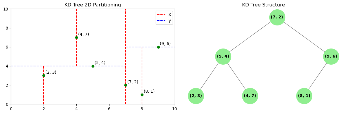
二维数据 KD 树空间划分示意图

KD 树的构建实现代码 理解流程

# Try to run this code on your local machine! ^_^

import matplotlib.pyplot as plt
import networkx as nx
import numpy as np

class Node:
    def __init__(self, point, left=None, right=None):
        self.point = point  # 当前节点的点
        self.left = left    # 左子树
        self.right = right  # 右子树
        

def choose_split_axis(points):
    points_np = np.array(points)  
    variances = np.var(points_np, axis=0)
    return np.argmax(variances) # 计算每个维度的方差，并返回最大的索引


# 构建 KD 树
def build_kd_tree(points, depth=0):
    if not points:
        return None

    # 根据最大方差选择轴
    axis = choose_split_axis(points)    // [!code ++]

    # 按照当前轴排序并选择中位数点
    points.sort(key=lambda x: x[axis])  
    median = len(points) // 2   

    return Node(
        point=points[median],
        left=build_kd_tree(points[:median], depth + 1),
        right=build_kd_tree(points[median + 1:], depth + 1)
    )


# 生成划分图
def plot_kd_tree(node, depth=0, min_x=0, max_x=10, min_y=0, max_y=10, ax=None):
    if node is None:
        return
    
    x, y = node.point
    axis = depth % 2
    
    if axis == 0:
        # 垂直分割
        ax.plot([x, x], [min_y, max_y], 'r--', label='x')
        plot_kd_tree(node.left, depth + 1, min_x, x, min_y, max_y, ax)
        plot_kd_tree(node.right, depth + 1, x, max_x, min_y, max_y, ax)
    else:
        # 水平分割
        ax.plot([min_x, max_x], [y, y], 'b--', label='y')
        plot_kd_tree(node.left, depth + 1, min_x, max_x, min_y, y, ax)
        plot_kd_tree(node.right, depth + 1, min_x, max_x, y, max_y, ax)

    # 绘制节点
    ax.plot(x, y, 'go')
    ax.text(x + 0.1, y + 0.2, f'({x:.f}, {y:.f})', fontsize=10, color='black')
    

# 生成树形图
def plot_kd_tree_networkx(node, graph=None, parent=None, pos=None, x=0, y=0, level_width=0.5, vertical_gap=1):
    if graph is None:
        graph = nx.DiGraph()
    if pos is None:
        pos = {}
    
    if node is not None:
        current_label = f"({node.point[0]:.0f}, {node.point[1]:.0f})"
        graph.add_node(current_label)
        pos[current_label] = (x, y)
        
        if parent is not None:
            graph.add_edge(parent, current_label)
        
        new_x_left = x - level_width
        new_x_right = x + level_width
        
        plot_kd_tree_networkx(node.left, graph, current_label, pos, new_x_left, y - vertical_gap, level_width / 2, vertical_gap)
        plot_kd_tree_networkx(node.right, graph, current_label, pos, new_x_right, y - vertical_gap, level_width / 2, vertical_gap)
    
    return graph, pos


# 建树
points = [(2,3), (5,4) , (9,6) , (4,7) , (8,1) ,(7,2)]
kd_tree = build_kd_tree(points)

# 画图
fig, (ax1, ax2) = plt.subplots(1, 2, figsize=(12, 4))
ax1.set_xlim(0, 10)
ax1.set_ylim(0, 10)
ax1.set_title("KD Tree 2D Partitioning")
plot_kd_tree(kd_tree, ax=ax1)
handles, labels = ax1.get_legend_handles_labels()
unique_labels = dict(zip(labels, handles))
ax1.legend(unique_labels.values(), unique_labels.keys())

ax2.set_title("KD Tree Structure")
graph, pos = plot_kd_tree_networkx(kd_tree)
nx.draw(graph, pos, with_labels=True, node_size=1500, node_color="lightgreen", font_size=10, font_weight='bold', edge_color="gray", arrows=False)
plt.tight_layout()
plt.show()

当进行近邻搜索时，我们可以通过递归地向下搜索 KD 树，主要流程如下：

• 当到达一个叶子结点，即得到最邻近的近似点，判断其是否为最优，并保存为“当前最优”；
• 回溯：对整棵树进行递归，并对每个结点执行以下操作“：
  • 如果当前结点比“当前最优”更近，替换为新的“当前最优”；
  • 判断分割平面的另一侧是否存在比“当前最优”更优的点。构造一个超球面，球心为查询点，半径为与当前最优的距离：
    • 如果超球面跟超平面相交，则有可能存在更优的点；按照相同的搜索过程，从当前结点向下移动到该节点的另一个分支以寻找更近的点。
    • 如果超球面跟超平面不相交，则沿着树继续往上走，当前结点的另一个分支则被排除。

例如，在上面的例子中，我们如果要查询点 $(2.1,3.1)$，显然，在第一次搜索时，我们很快就能找到最右边的叶子结点 $(2,3)$，此时的欧式距离为 $0.1\sqrt{2}$。然后我们回溯到点 $(5,4)$，其分割“平面”（即直线 $y=4$）与“超球面”（即圆 $(x-2.1{)}^2+(y-3.1{)}^2=(0.1\sqrt{2}{)}^2$）不相交。因此，我们可以继续向上回溯，不必再访问 $(5,4)$ 的右子树（这一步时，如果平面与球面相交，则需要进入右分支寻找更近点，在回溯时，如果遇到更近点点需要及时更新）。直到访问到根节点后，我们可以得到最近邻点 $(2,3)$。

KD 树的查询实现代码 理解流程

首先，我们定义函数 euclidean_distance 来计算两个点之间的欧式距离。然后，我们定义函数 find_nearest_neighbor 来寻找最近邻点。

# Try to run this code on your local machine! ^_^
# Warning: You have to combine this code
# with the previous KD-tree-building code
# in order to run it successfully.

def euclidean_distance(point1, point2):
    return np.linalg.norm(np.array(point1) - np.array(point2))


def find_nearest_neighbor(node, target, depth=0, best=None):
    if node is None:
        return best
    
    # 更新当前最优解
    distance = euclidean_distance(node.point, target)
    if best is None or distance < best[0]:
        best = (distance, node.point)

    # 判断分割轴并选择搜索方向
    axis = depth % 2
    next_branch = None
    opposite_branch = None

    if target[axis] < node.point[axis]:
        next_branch = node.left
        opposite_branch = node.right
    else:
        next_branch = node.right
        opposite_branch = node.left

    # 向下搜索下一分支
    best = find_nearest_neighbor(next_branch, target, depth + 1, best)

    # 判断超球面与分割平面是否相交，若相交，则寻找另一分支
    if abs(target[axis] - node.point[axis]) < best[0]:
        best = find_nearest_neighbor(opposite_branch, target, depth + 1, best)

    # 回溯
    return best

接下来，我们可以寻找最近邻点。

target_point = (2.1, 3.1)
nearest_neighbor = find_nearest_neighbor(kd_tree, target_point)

print(f"Nearest neighbor to {target_point} is {nearest_neighbor[1]} with distance {nearest_neighbor[0]:.4f}")

程序的输出为：

Nearest neighbor to (2.1, 3.1) is (2, 3) with distance 0.1414

KD 树的查询复杂度为 $O(n\log n)$，其中查找中位数的复杂度为 $O(n)$，而在树上寻找最近邻点的复杂度为 $O(\log n)$。

其他方法

另一种方法是对数据进行降维。它的核心思想是通过某种数学变换将原式高位属性空间转变为低维子空间，来化解维数灾难问题。主要的方法有：

• 多维缩放算法
• 主成分分析
• 局部线性潜入
• Isomap 算法等

哈希也是一种降维的手段。哈希的核心思想是利用哈希函数把任意长度的输入映射为固定长度的输出。

此外，近似最近邻也是一种可行的方法。它的核心思想搜索可能是近邻的数据项而不再只局限于返回最可能的数据项，在牺牲可接受范围内的精度的情况下提高检索效率。

扩展阅读

$k-NN$ 算法的缺点是它并不建立在任何概率框架上，所以无法得到关于类别的后验概率。我们可以通过定义似然函数来构造关于概率的 $k-NN$ 算法。具体可以参考这篇论文。