Turing Machine

The purpose of the theory of Turing machines is to prove that whether a certain specific language have algorithmic solution or not. We will introduce the concept of Turing machines and their properties.

Definition of Turing Machine

We first have a look at the picture of a Turing machine.

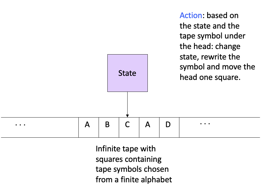
A Turing Machine

We have a tape and a head that can move left or right on the tape. The tape, which is divided into cells, is infinite in both directions. The head itself has a finite number of states, which can change based on the current state and the symbol it reads on the tape. The head can also write symbols on the tape based on its state.

A Turing machine can be formally defined as a 7-tuple $(Q,\mathrm{\Sigma },\mathrm{\Gamma },\delta ,q_0,q_{\text{accept}},q_{\text{reject}})$:

• $Q$ is a finite set of states.
• $\mathrm{\Sigma }$ is the input alphabet, which does not contain the blank symbol $\bigsqcup$.
• $\mathrm{\Gamma }$ is the tape alphabet, which contains $\mathrm{\Sigma }$ and the blank symbol $\bigsqcup$.
• $\delta :Q\times \mathrm{\Gamma }\to Q\times \mathrm{\Gamma }\times \{L,R,H\}$ is the transition function.
• $q_0\in Q$ is the start state.
• $q_{\text{accept}}\in Q$ is the accept state.
• $q_{\text{reject}}\in Q$ is the reject state.

Why Turing Machine?

Why not we just use C program or Python program? The answer is that you can, but it is easier to prove things with Turing machines. The Turing machine is a theoretical model of computation, which is simple and powerful. What's more, it is equivalent to any other model of computation and its memory is free of charge!

Transition Function

The transition function $\delta$ is defined as $\delta :Q\times \mathrm{\Gamma }\to Q\times \mathrm{\Gamma }\times \{L,R,H\}$. It means that the Turing machine can change its state, write a symbol on the tape, and move the head to left($L$) cell or right($R$) cell. The head can also hold still($H$).

For example, if the Turing machine is in state $q$ and reads symbol $a$ on the tape, then it can change to state $q^{\prime }$, write symbol $b$ on the tape, and move the head to the right cell. The transition can be denoted as $\delta (q,a)=(q^{\prime },b,R)$.

Instantaneous Description

We can also take a photo of the Turing machine at a certain moment, which is called the instantaneous description. It is denoted as $uqv$, where $u$ is the left part of the tape, $v$ is the right part of the tape, and $q$ is the current state. The head is pointing to the first symbol of $v$. The actual tape is $uv$, with infinite $\bigsqcup$ on both sides.

Then we can have the following transition:

• If $\delta (q,X)=(q^{\prime },Y,R)$, then $\alpha qX\beta ⊢\alpha Y{q}^{\prime }\beta$.
• If $\delta (q,X)=(q^{\prime },Y,L)$, then $\alpha ZqX\beta ⊢\alpha q^{\prime }ZY\beta$. (Of course, $qX\beta ⊢q^{\prime }\bigsqcup Y\beta$)

We can also define ${⊢}^{\ast }$ as multiple transitions in a row.

Language of a Turing Machine

A Turing machine $M$ can accept a language by final state, which is denoted as $L(M)=\{w\mid q_{0}w{⊢}^{\ast }\alpha q_{\text{accept}}\beta \}$. Or, it can accept a language by halting, which is denoted as $H(M)=\{w\mid q_{0}w{⊢}^{\ast }I\}$, where $I$ is an instantaneous description that cannot be further transitioned.

Do we have to eat the whole string?

We don't need to consume the whole input string in a Turing machine to accept it. The Turing machine can accept the string by halting or reaching final state at any moment. This is different from the PDA, which must consume the whole string to accept it.

Equivalence of Acceptance

We can prove that each $L(M)$ has a corresponding $H(M^{\prime })$.

Proof

( From $L(M)$ to $H(M^{\prime })$ ) For each final state of $M$, remove any moves, then the result $M^{\prime }$ must halt at that point. On the other hand, we have to prevent $M^{\prime }$ from accidentally halting at other points. We can add a new state $q_{\text{inf}}$ to make any turing machine that reaches $q_{\text{inf}}$ to loop endlessly (e.g., adding a transition function $\delta (q_{\text{inf}},X)=(q_{\text{inf}},X,R)$ for any $X$). If a non-accepting state reaches no state, then we add one transition to $q_{\text{inf}}$.

( From $H(M)$ to $L(M^{\prime })$ ) We introduce a new state $f$, the only accepting state in $M^{\prime }$. $f$ has no transitions. If $\delta (q,X)$ is undefined for any $q$ and $X$, then we add a transition $\delta (q,X)=(f,X,R)$.

Recursive and Recursively Enumerable Languages

The Turing machine can accept languages in two ways: by final state or by halting. And we now know the two language are equivalent. Thus, we define this set of languages as recursively enumerable languages. This term has a long history and don't be confused by the name. Almost all languages we can think of are recursively enumerable.

An algorithm $M$ is a Turing machine, accepting at accept state and rejecting at reject state. In all, it will always halt.

If $L=L(M)$ for some algorithm $M$, we say $L$ is a recursive language.

We can conclude that:

• Recursive: Accept (string in the language) or Reject (string not in the language). (Or, Halt or Loop)
• Recursively Enumerable: Accept (string in the language), Reject or Loop (string not in the language).

Closure Properties

Both recursive and recursively enumerable languages have the following closure properties:

• Union (Easy to show): If $L_1$ and $L_2$ are recursive (or recursively enumerable), then $L_1\cup L_2$ is recursive (or recursively enumerable).
• Intersection (Easy to show): If $L_1$ and $L_2$ are recursive (or recursively enumerable), then $L_1\cap L_2$ is recursive (or recursively enumerable).
• Concatenation: If $L_1$ and $L_2$ are recursive (or recursively enumerable), then $L_1\cdot L_2$ is recursive (or recursively enumerable).
• Kleene Star: If $L$ is recursive (or recursively enumerable), then $L^{\ast }$ is recursive (or recursively enumerable).
• Reverse: If $L$ is recursive (or recursively enumerable), then $L^R$ is recursive (or recursively enumerable).
• Inverse Homomorphism: If $L$ is recursive (or recursively enumerable), then $h(L)$ is recursive (or recursively enumerable), where $h$ is a homomorphism.

Proof of Closure Properties

Concatenation: For recursive enumerable language $L_1$ and $L_2$, we can construct a Turing machine $M_1$ and $M_2$ to accept $L_1$ and $L_2$ respectively. Then, on one input $x$, we can iterate all possible ways to split $x$ into $x_1$ and $x_2$, and run $M_1$ on $x_1$ and $M_2$ on $x_2$, separately. If one of them both accepts, then accept. (If in one of the iteration, both $M_1$ and $M_2$ loop, then the entire machine loops.) Apparently, recursive languages, Kleene Star can be proved in a similar way.

Reverse: We can first reverse the input string and run the Turing machine on it.

Only recursive languages have the following closure properties:

• Difference: If $L_1$ and $L_2$ are recursive, then $L_1-L_2$ is recursive.
• Complement: If $L$ is recursive, then $\bar{L}$ is recursive.

No complement in RE

If $L$ is recursively enumerable and $\bar{L}$ is also recursively enumerable, then $L$ is recursive. But the set of recursive languages is a proper subset of recursively enumerable languages. Thus, RE is not closed under complement.

However, the complement of RE is called $\text{co-RE}$, we will talk about it in the next section.

But RE is under the closure of homomorphism.

No homomorphism in recursive languages

Consider a Turing machine whose language $L$ is RE. We define a homomorphism $h$, which maps the transition chain of string $s$ on that TM (denoted as a string) to the string $s$ itself. Apparently, all the strings of transition chains (language $L^{\prime }$) are recursive (easy to decide whether the transition is valid), yet the original language $L$ is RE. Thus, we found a counterexample $h:L^{\prime }\to L$, where $L^{\prime }$ is recursive and $L$ is RE.

Read more here.

Turing Machine Programming

We know that recursively enumerable languages are powerful, so is the Turing machine. Generally, unlike former DFA or PDA, Turing machine is not used to recognize languages, but to compute functions, which is related to programming.

Let's have a look at the following example:

Example 1 Construct a Turing Machine to recognize the language $L=\{a^n{b}^n\mid n\ge 0\}$.

Solution 1 We can construct a Turing machine as follows:

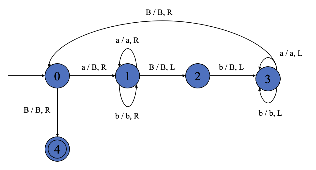
The graph of solution 1

The transitions are shown on the graph above. Note that the sign $a/b,R$ on each transition means that the machine reads $a$ and writes $b$ on the tape, then moves the head to the right cell.

Suppose the input string is $S$, this Turing machine runs as the following pseudocode:

while( S != "" ) {
    if(S[0] == 'a') {
        S.erase(0, 1);
    }else{
        reject;
    }
    if(S[S.size()-1] == 'b') {
        S.erase(S.size()-1, 1);
    }else{
        reject;
    }
}
accept;

Example 2 Construct a Turing Machine to shift each input symbol one cell to the right, while the leftmost symbol is replaced by $\bigsqcup$.

Solution 2 We can construct a Turing machine as follows:

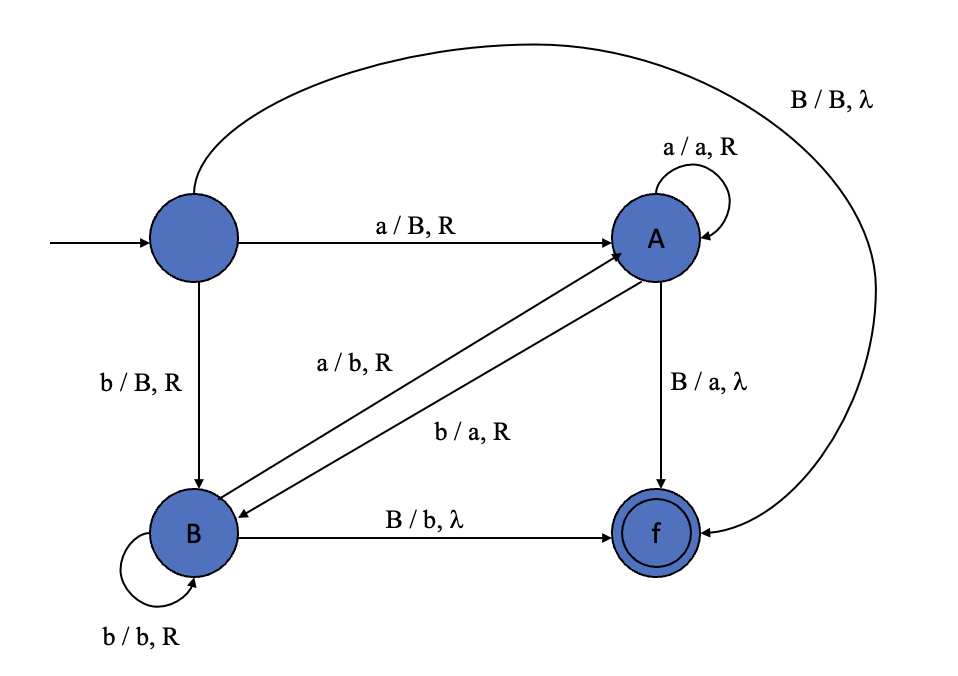
The graph of solution 2

Example 3 Construct a Turing Machine to shift its words cyclically to the right.

Solution 3 We can construct a Turing machine as follows:

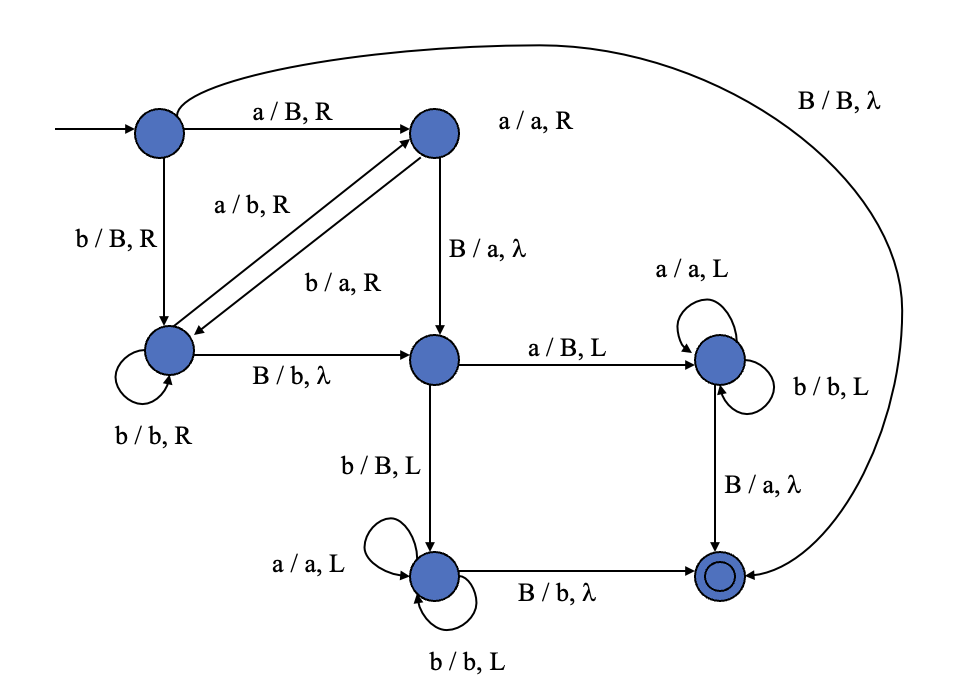
The graph of solution 2

Note that the upper-left corner of the graph is the same as the graph in solution 2, and the lower-right corner is to write the last symbol to the first cell. We can perceive this idea of constructing turing machine as structured programming.

Example 4 (Decider) Let $L=\{b{a}^{i}b\mid i\ge 0\}$, construct a Turing Machine to decide $L$. You have to give the result on the tape in order to decide.

Solution 4 Trivially, we can construct a Turing machine without decider as follows:

A prototype of solution 4

Then, we can add a decider to the Turing machine as shown below:

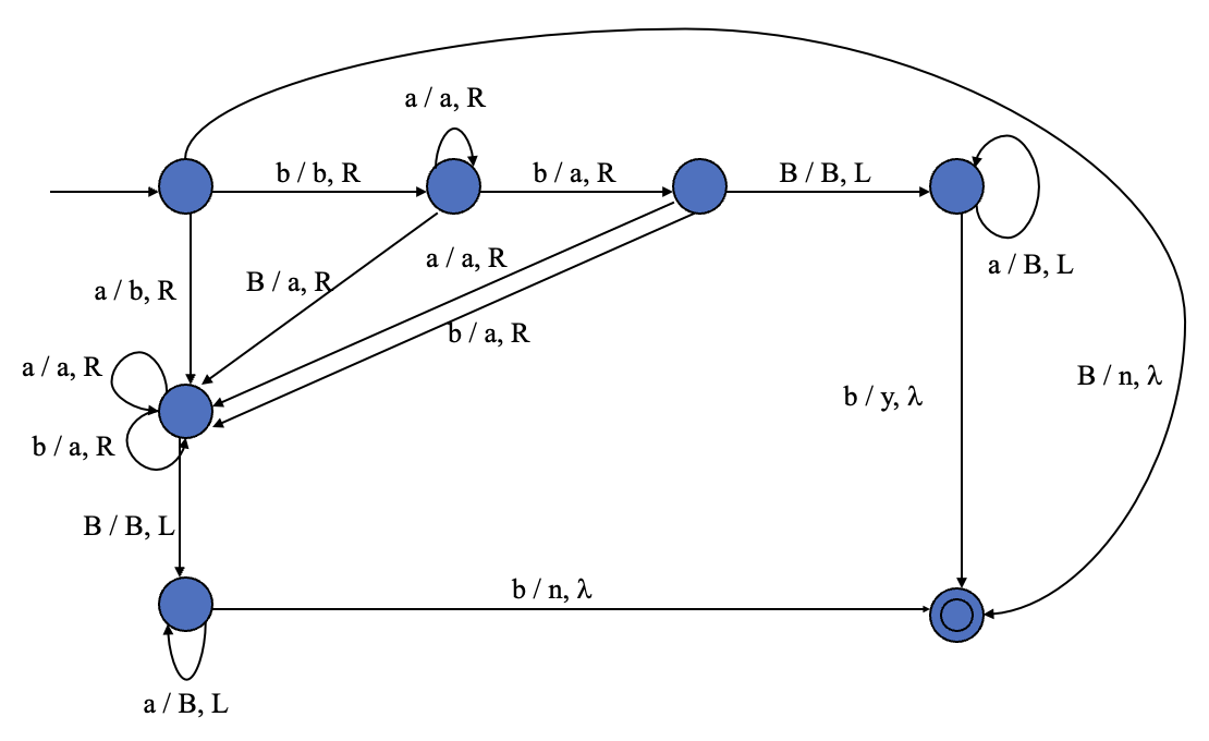
The graph of solution 4

The decider makes its way to the leftmost cell, modifying all the cells to blank symbols along the way, then subsequently writes $y$ or $n$ on the tape to decide whether the input string is in the language.

Programming Tricks

Multiple Tracks

We can use the standard Turing machine to simulate a multi-track Turing machine. The machine still possesses only one tape, but each cell can store multiple symbols, as vector (or tuple, whatever you like). The head can read and write multiple symbols at once.

We can use the symbol $[a,b,c]$ to denote the vector, where $a,b,c$ are the symbols on each track. The head can read and write the vector $[a,b,c]$ at once. We use $[\bigsqcup ,\cdots ,\bigsqcup ]$ to denote blank symbol. The transition function can be defined as $\delta :Q\times {\mathrm{\Gamma }}^k\to Q\times {\mathrm{\Gamma }}^k\times \{L,R,H\}$, where $k$ is the number of tracks.

Marker

Using the trick of multiple tracks, we can make one extra track the marker track. Almost all the cells on the marker track are blank symbols, but few are marked with a special symbol (Marker) to indicate some information.

Extensions

There are many extensions of Turing machines, which are more general than the standard Turing machine. However, they are all equivalent to the standard Turing machine, but more intuitive and easier to use. Here are some of them:

• Semi-infinite Turing machine
• Multi-tape Turing machine
• Non-deterministic Turing machine

Semi-infinite Turing Machine

A semi-infinite Turing machine has a semi-infinite tape, which is infinite in one direction (usually right) and finite in the other.

We can use multi-track Turing Machine to simulate it. Just imagine the infinite track being folded into a semi-infinite tape, denoting by one upper track and lower track. The machine can remember whether simulating the upper track or the lower track by the state. If simulating the lower track, the head moves the opposite direction to that in the previous infinite tape. If the head reaches the leftmost cell, it shifts its state to simulate the other track.

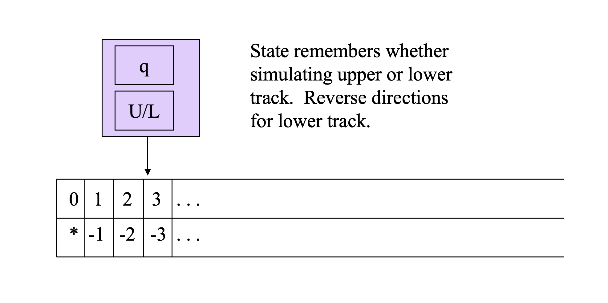
Simulating Semi-infinite TM

What about two stacks?

The semi-infinite tape is just like two stacks. Actually, we can even just use two stacks to simulate Turing machines.

We know, the ID of a Turing machine is $uqv$, where $u$ is the left part of the tape, $v$ is the head and the right part of the tape, and $q$ is the current state. We can use two stacks to store $u$ and $v$, and the head is the top of the second stack. The state of the Turing machine is the state of the stack machine (like PDA).

Multi-tape Turing Machine

Difference between Multi-tape and Multi-track

The multi-tape Turing machine has multiple tapes, and the heads can move independently. The multi-track Turing machine has only one tape, but each cell can store multiple symbols.

We can show that all multi-tape Turing machines can be simulated by a single-tape & multi-track Turing machine. A simple idea is that: for a $k$-tape Turing machine, we could use a $2k$-track Turing machine to simulate it. The first $k$ tracks are used to simulate the tapes, and the other $k$ tracks are used to simulate the heads (There are only one symbol on each track, which denotes the position of the head).

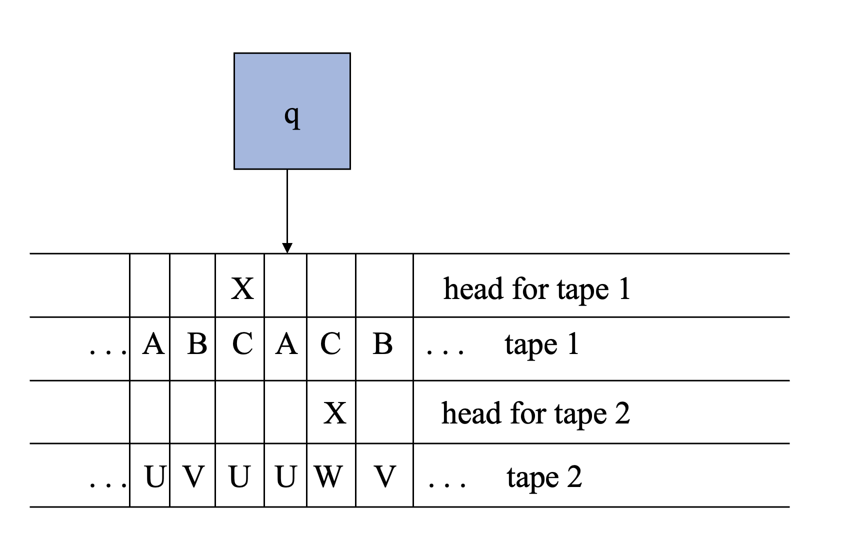
Simulating Multi-Tape TM

Non-deterministic Turing Machine

As NFAs, non-deterministic Turing machines can have multiple transitions for a single state and symbol. The machine accepts the input string if there exists a path that leads to an accepting state.

The non-deterministic Turing machine is equivalent to the deterministic Turing machine. We can convert a non-deterministic Turing machine to a deterministic Turing machine by breadth-first search.

Converting an NTM

We can convert an NTM (non-deterministic Turing machine) to a multi-track DTM by using the idea of BFS. The DTM has two tracks:

• One track records a queue of ID's of the NTM.
• The other track is used to mark certain positions. One mark denotes the current state of the NTM, which is the head of the queue. The other mark help to simulate the transitions of the NTM, adding one-move change to the rear of the queue.

Then, we can use the DTM to simulate the NTM by breadth-first search.

The DTM derived from the NTM does have an upper bound of the size of states and queue. Let the upper bound of numbers of the moving-choices of the NTM be $k$, then any ID reachable from the initial ID by $n$ moves will be constructed in the DTM after constructing at most $(k^{n+1}-k)/(k-1)$ ID's.